Class 10 : Maths (In English) – Lesson 13. Statistics

EXPLANATION & SUMMARY

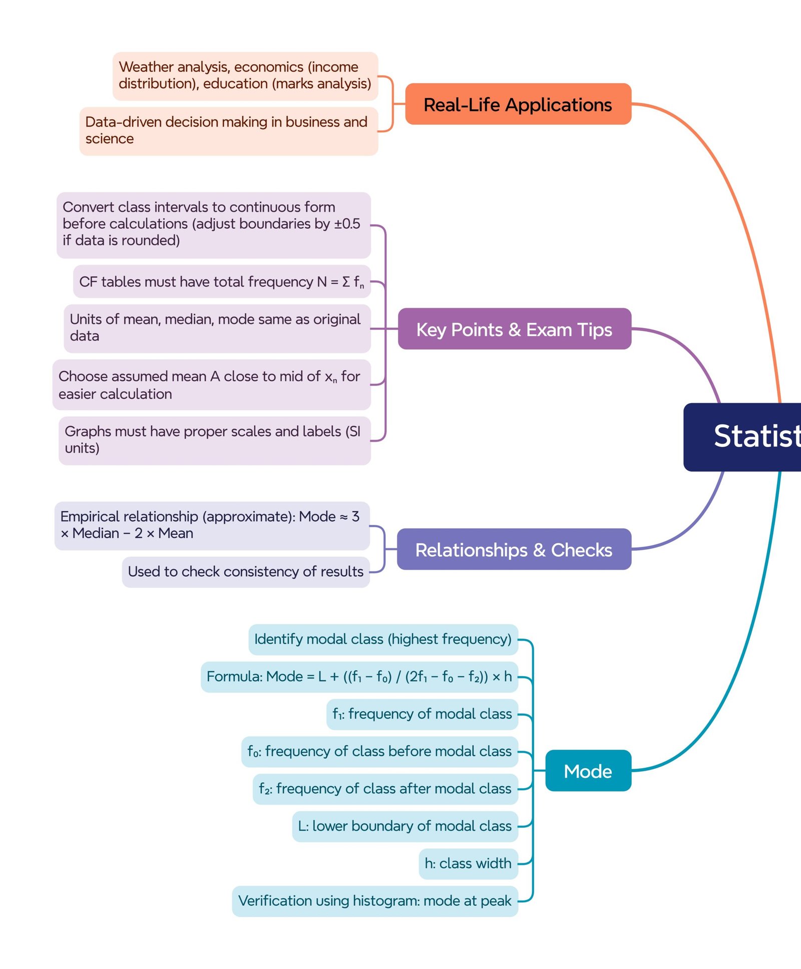
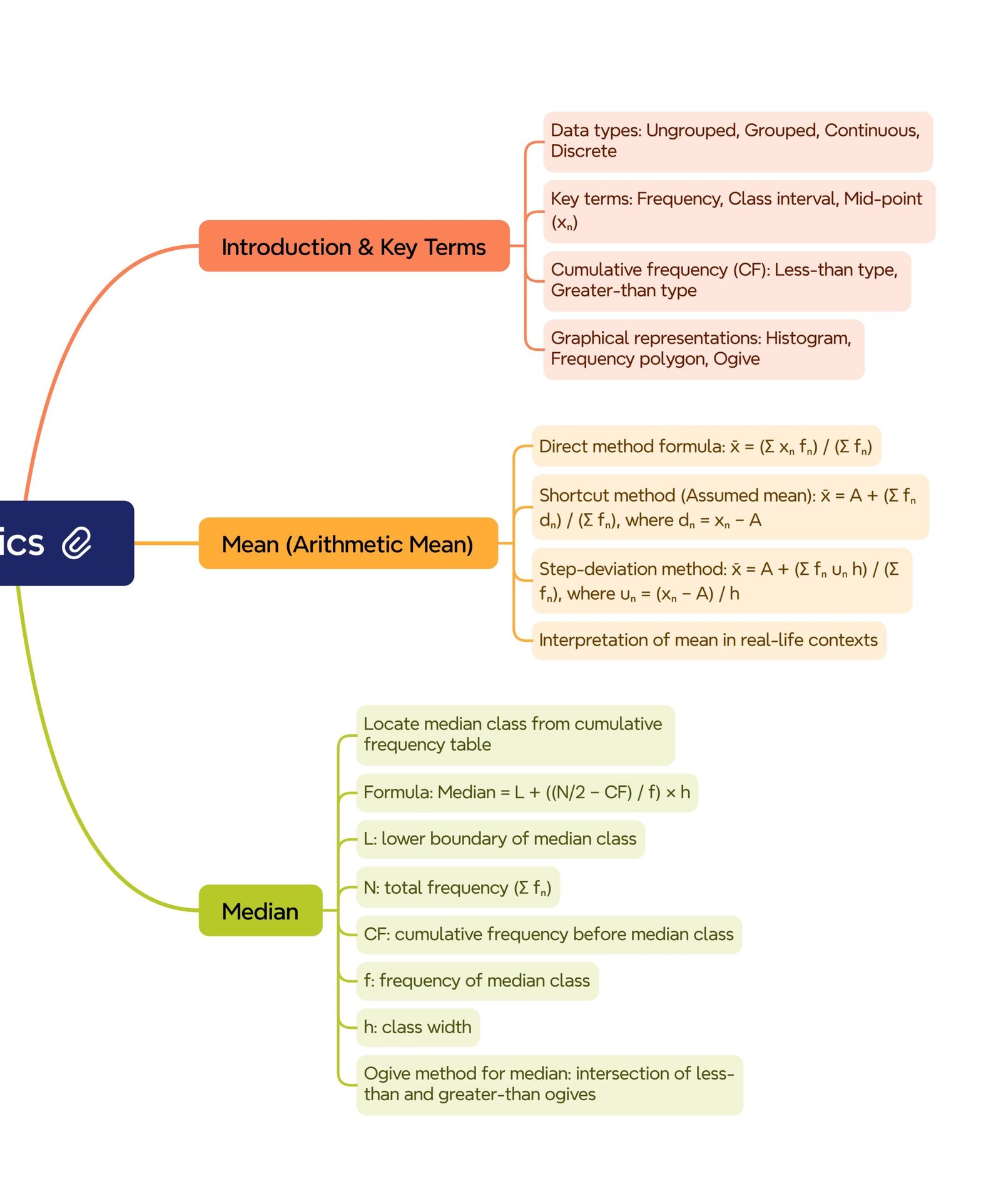
🔵 Introduction
• 📚 Statistics is the science of collecting, organizing, presenting, analyzing, and interpreting numerical data.
• 🧭 In Class 10, you will:
 🔹 Construct grouped frequency distributions
 🔹 Draw histograms, frequency polygons, and ogives
 🔹 Calculate mean, median, and mode for grouped data
 🔹 Apply these ideas to real-life contexts like exam marks, rainfall data, or business trends.
✏️ Note: Exclude highlighted boxes or tables from NCERT.

🟢 1️⃣ Understanding Data and Frequency Distributions
🔴 Raw data are unsorted observations—for example, marks of forty students.
🟡 Frequency means how many times a particular value or class occurs.
🔵 Class intervals are continuous ranges like 0–10, 10–20, 20–30.
🟢 Class marks are midpoints: add the lower and upper limits then divide by 2.
💡 Concept Tip: Always choose equal widths (like 5 or 10) to keep computation simple.
✔️ Exclusive method: The upper class limit is not included in that interval—for instance, 10 belongs to 10–20, not 0–10.
➡️ Example frequencies inline: Suppose marks are grouped as 0–10 (5 students), 10–20 (10 students), 20–30 (20 students), 30–40 (10 students), and 40–50 (5 students). The total number of students is 50.

🟠 2️⃣ Graphical Representation of Data
(a) 📈 Histograms
1️⃣ Draw the x-axis for class intervals.
2️⃣ Draw the y-axis for frequencies.
3️⃣ Plot adjacent bars of equal width—no gaps between them.
4️⃣ Label axes and give a title.
✏️ Note: If intervals are unequal, convert frequencies to frequency densities by dividing each frequency by its class width before plotting.
(b) 🔵 Frequency Polygons
• Draw the histogram first, mark the midpoints at the top of each bar, and join them with straight lines.
• Alternatively, plot class midpoints with frequencies directly and connect them. Close the polygon by linking to zero-frequency points at each end.
(c) 🟡 Ogives (Cumulative Frequency Curves)
• A less-than ogive plots each upper class boundary with its cumulative frequency.
• A more-than ogive plots each lower class boundary with cumulative frequencies counted downward.
💡 Tip: The intersection of less-than and more-than ogives approximates the median graphically.

🔵 3️⃣ Measures of Central Tendency – Mean, Median, Mode
🟢 (a) Mean of Grouped Data
Formula: x̄ = Σ(fᵢ × xᵢ) ÷ Σfᵢ
➡️ Example without table: Take the earlier data—class marks are 5, 15, 25, 35, 45 and frequencies are 5, 10, 20, 10, 5. Multiply each: 5×5 = 25, 10×15 = 150, 20×25 = 500, 10×35 = 350, 5×45 = 225. Sum frequencies = 50. Sum of products = 1250. Mean x̄ = 1250 ÷ 50 = 25.
✏️ Note: Use the assumed mean or step deviation method to simplify when numbers are large.
🟡 (b) Median of Grouped Data
Formula: Median = L + ((N/2 – CF) ÷ f) × h
➡️ Using the same data: cumulative frequencies are 5, 15, 35, 45, 50. N = 50, N/2 = 25. The median class is 20–30 (L = 20, CF = 15, f = 20, h = 10). Median = 20 + ((25 – 15)/20) × 10 = 25.
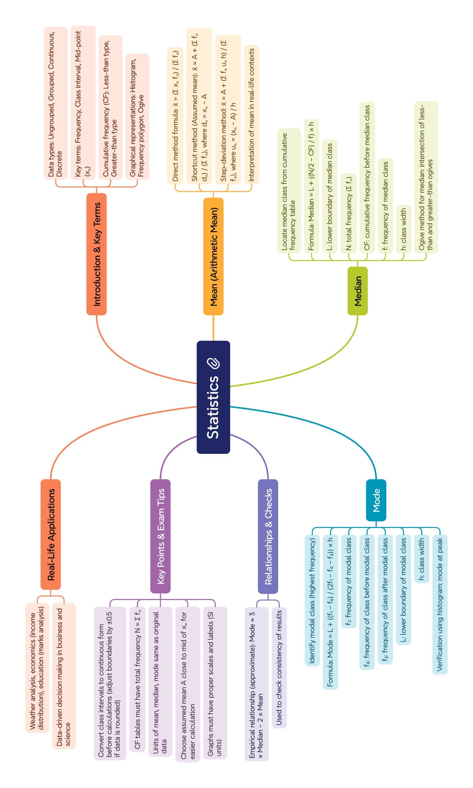
🔴 (c) Mode of Grouped Data
Formula: Mode = L + ((f₁ – f₀)/(2f₁ – f₀ – f₂)) × h
➡️ For modal class 20–30: f₁ = 20, f₀ = 10, f₂ = 10, L = 20, h = 10. Mode = 20 + ((20–10)/(40–10–10)) × 10 = 25.

🟠 4️⃣ More Worked Examples
📐 Example 1: Mean Using Assumed Mean Method
Class intervals: 10–20 (5), 20–30 (8), 30–40 (12), 40–50 (15), 50–60 (10). Midpoints: 15, 25, 35, 45, 55. Choose assumed mean A = 35 and class width h = 10. Differences: 15–35 = –20 (d = –2), 25–35 = –10 (d = –1), 35–35 = 0, 45–35 = 10 (d = 1), 55–35 = 20 (d = 2). Multiply frequencies and d values: 5×–2 = –10, 8×–1 = –8, 12×0 = 0, 15×1 = 15, 10×2 = 20. Sum f = 50, sum f×d = 17. Mean = A + (Σfᵢdᵢ/Σfᵢ)×h = 35 + (17/50)×10 = 38.4.
📊 Example 2: Median Using Ogive
Class intervals: 0–20 (7), 20–40 (10), 40–60 (20), 60–80 (9), 80–100 (4). N = 50 ⇒ N/2 = 25. Cumulative frequencies: 7, 17, 37, 46, 50. Median class = 40–60 (L = 40, CF = 17, f = 20, h = 20). Median = 40 + ((25 – 17)/20) × 20 = 48.
📏 Example 3: Mode via Formula
For 30–40 as modal class: f₁ = 18, f₀ = 12, f₂ = 10, L = 30, h = 10. Mode = 30 + ((18 – 12)/(36 – 12 – 10)) × 10 = 34.29.

🔵 5️⃣ Applications of Statistics
• 📈 Education – Comparing students’ test scores.
• 🛒 Business – Forecasting demand from sales figures.
• 🌦 Meteorology – Analyzing rainfall or temperature patterns.
• 🧭 Government Planning – Studying population data for resource allocation.
• 🏀 Sports – Evaluating player performance through averages.

🟡 6️⃣ Common Mistakes and Precautions
🔴 Overlapping class intervals (counting boundary values twice).
🟢 Forgetting to adjust frequencies for unequal widths.
🔵 Miscalculating cumulative frequencies before the median class.
🟡 Rounding too early—retain at least two decimals until the final step.
✏️ Note: Always check that the sum of frequencies matches the total number of observations.

🟢 7️⃣ Advanced Technique – Step Deviation Method
Formula: x̄ = A + (Σfᵢdᵢ ÷ Σfᵢ) × h
• A is an assumed mean chosen near the center.
• dᵢ = (xᵢ – A)/h.
• h is class width.
💡 Tip: Keeping dᵢ values small speeds calculations and reduces errors.

🟠 8️⃣ Graphical Comparisons
• Overlay multiple frequency polygons on the same axes to compare two data sets.
• Draw double ogives to contrast cumulative trends.
• Combine histogram and polygon for deeper insights into distribution shapes.

🔴 9️⃣ Extended Real-Life Example
Monthly salaries of employees in thousands of rupees:
Classes = 0–10 (3 employees), 10–20 (7), 20–30 (12), 30–40 (18), 40–50 (10).
Mean: midpoints = 5, 15, 25, 35, 45. Products = 15, 105, 300, 630, 450. Sum frequencies = 50. Sum products = 1500. Mean = 1500 ÷ 50 = 30 k.
Median: cumulative frequencies = 3, 10, 22, 40, 50. Median class = 30–40 (L = 30, CF = 22, f = 18, h = 10). Median = 30 + ((25 – 22)/18) × 10 = 31.67 k.
Mode: modal class = 30–40 (f₁ = 18, f₀ = 12, f₂ = 10). Mode = 30 + ((18 – 12)/(36 – 12 – 10))×10 = 34.29 k.

🟢 1️⃣0️⃣ Why Use All Three Measures
• Mean shows the overall average but is sensitive to outliers.
• Median resists extremes—good for skewed data.
• Mode highlights the most common value—helpful in marketing or quality control.
✏️ Note: Use them together for a fuller picture.

🟠 1️⃣1️⃣ Recap of Graph Types
• Histogram: x-axis for class bounds, y-axis for frequency—shows distribution shape.
• Frequency polygon: x-axis for midpoints, y-axis for frequency—useful for comparison.
• Less-than ogive: x-axis upper bound, y-axis cumulative frequency—find median graphically.
• More-than ogive: x-axis lower bound, y-axis cumulative frequency—compare trends.

🟡 1️⃣2️⃣ Extra Tips
• Verify Σfᵢ equals total observations.
• Label axes clearly and add descriptive titles.
• Choose convenient class widths that divide the range evenly.
• Cross-check means with calculators to avoid arithmetic mistakes.
• Use smooth curves for ogives to improve readability.

✨ Summary (~300 words)
Statistics organizes raw numbers into patterns. Data are grouped into frequency distributions where each class interval has an associated frequency. Using equal widths and exclusive classes prevents overlap. Tallying makes counting efficient.
Visual representation is essential: Histograms show adjacent bars of frequency, frequency polygons connect midpoints, and ogives plot cumulative frequencies to reveal medians. Graphs quickly reveal trends and comparisons.
Three measures of central tendency summarize data:
• Mean (Σfᵢxᵢ ÷ Σfᵢ) is the arithmetic average but can be distorted by extreme values.
• Median (L + ((N/2 – CF)/f) × h) splits data into two equal halves and resists outliers.
• Mode (L + ((f₁–f₀)/(2f₁–f₀–f₂)) × h) identifies the most frequent class. Graphical checks like ogive intersections and histogram parallelograms confirm these measures.
Applications span education, economics, meteorology, sports, and business. For example, teachers analyze exam results, businesses forecast sales, meteorologists study rainfall, and governments plan resources.
Common mistakes—overlapping intervals, incorrect cumulative frequencies, or premature rounding—can mislead. Always check Σfᵢ totals, choose sensible class widths, and retain two decimals until the final step.
Using all three measures (mean, median, and mode) together gives a balanced understanding of data. Histograms, polygons, and ogives enrich interpretation, making statistics an indispensable tool for decision-making.

📝 Quick Recap
• 📊 Organize raw data into frequency distributions.
• ➡️ Draw histograms, polygons, and ogives for clear visuals.
• ➡️ Mean = Σ(fᵢxᵢ) ÷ Σfᵢ.
• ➡️ Median = L + ((N/2 – CF) ÷ f) × h.
• ➡️ Mode = L + ((f₁–f₀)/(2f₁–f₀–f₂)) × h.
• 🧭 Median via ogive intersection, mode via histogram method.
• ✔️ Apply statistics in education, business, weather, sports, and planning.
• ⚠️ Avoid overlapping intervals and rounding too early.

———————————————————————————————————————————————————————————————————————————–

TEXT BOOK QUESTIONS

Exercise 13.1

🟢 Question 1
🔸 Q: A survey was conducted … number of plants in 20 houses … Find the mean number of plants per house. Which method did you use and why?
🔸 Classes: 0–2, 2–4, 4–6, 6–8, 8–10, 10–12, 12–14
🔸 Frequencies (fᵢ): 1, 2, 1, 5, 6, 2, 3
Solution
1️⃣ Midpoints (xᵢ): 1, 3, 5, 7, 9, 11, 13
2️⃣ Choose assumed mean A = 7 for convenience, h = 2.
3️⃣ Compute dᵢ = (xᵢ – A)/h → –3, –2, –1, 0, 1, 2, 3.
4️⃣ Multiply fᵢ·dᵢ: –3, –4, –1, 0, 6, 4, 9 → Σ(fᵢ·dᵢ)=11.
5️⃣ Σfᵢ = 20.
➡️ Mean = A + (Σfᵢ·dᵢ/Σfᵢ)×h = 7 + (11/20)×2 = 7 + 1.1 = 8.1 plants.
✔️ Used step deviation method because class width is equal and midpoints are convenient.

🟢 Question 2
🔸 Q: Daily wages (₹): 500–520, 520–540, 540–560, 560–580, 580–600.
Frequencies: 12, 14, 8, 6, 10.
Solution
1️⃣ Midpoints: 510, 530, 550, 570, 590.
2️⃣ Take assumed mean A = 550, h = 20.
3️⃣ dᵢ: –2, –1, 0, 1, 2.
4️⃣ fᵢ·dᵢ: –24, –14, 0, 6, 20 → Σ(fᵢ·dᵢ)=–12.
5️⃣ Σfᵢ=50.
➡️ Mean = 550 + (–12/50)×20 = 550–4.8 = ₹545.2.
✔️ Step deviation chosen for simpler arithmetic.

🟢 Question 3
🔸 Q: Daily pocket allowance (₹): 11–13, 13–15, 15–17, 17–19, 19–21, 21–23, 23–25.
Frequencies: 7, 6, 9, 13, f, 5, 4. Mean = 18. Find f.
Solution
1️⃣ Midpoints: 12, 14, 16, 18, 20, 22, 24.
2️⃣ Multiply:
 7×12=84, 6×14=84, 9×16=144, 13×18=234, f×20=20f, 5×22=110, 4×24=96.
3️⃣ Σfᵢ = 44 + f.
4️⃣ Σ(fᵢxᵢ)=84+84+144+234+20f+110+96=752+20f.
5️⃣ Mean formula: 18 = (752+20f)/(44+f).
6️⃣ Cross multiply: 18(44+f)=752+20f → 792+18f=752+20f.
7️⃣ 792–752=20f–18f →40=2f →f=20.
✔️ Missing frequency = 20 children.

🟢 Question 4
🔸 Q: Heartbeats/minute classes: 65–68, 68–71, 71–74, 74–77, 77–80, 80–83, 83–86.
Frequencies: 2, 4, 3, 8, 7, 4, 2.
Solution
1️⃣ Midpoints: 66.5, 69.5, 72.5, 75.5, 78.5, 81.5, 84.5.
2️⃣ Assume A = 75.5, h=3.
3️⃣ dᵢ: –3, –2, –1, 0, 1, 2, 3.
4️⃣ fᵢ·dᵢ: –6, –8, –3, 0, 7, 8, 6 → Σ=4.
5️⃣ Σfᵢ=30.
➡️ Mean = 75.5 + (4/30)×3 = 75.5+0.4 = 75.9 beats/min.

🟢 Question 5
🔸 Q: Mango boxes classes: 50–52, 53–55, 56–58, 59–61, 62–64.
Frequencies: 15, 110, 135, 115, 25.
Solution
1️⃣ Midpoints: 51, 54, 57, 60, 63.
2️⃣ Choose A=57, h=3.
3️⃣ dᵢ: –2, –1, 0, 1, 2.
4️⃣ fᵢ·dᵢ: –30, –110, 0, 115, 50 → Σ=25.
5️⃣ Σfᵢ=400.
➡️ Mean = 57+(25/400)×3=57+0.1875=57.19 mangoes.

🟢 Question 6
🔸 Q: Daily food expenditure classes: 100–150, 150–200, 200–250, 250–300, 300–350.
Frequencies: 4, 5, 12, 2, 2.
Solution
1️⃣ Midpoints: 125, 175, 225, 275, 325.
2️⃣ A=225, h=50.
3️⃣ dᵢ: –2, –1, 0, 1, 2.
4️⃣ fᵢ·dᵢ: –8, –5, 0, 2, 4 → Σ=–7.
5️⃣ Σfᵢ=25.
➡️ Mean = 225+(–7/25)×50=225–14=₹211.

🟢 Question 7
🔸 Q: SO₂ concentration classes (ppm): 0.00–0.04, 0.04–0.08, 0.08–0.12, 0.12–0.16, 0.16–0.20, 0.20–0.24.
Frequencies: 4, 8, 9, 2, 4, 2.
Solution
1️⃣ Midpoints: 0.02, 0.06, 0.10, 0.14, 0.18, 0.22.
2️⃣ Assume A=0.10, h=0.04.
3️⃣ dᵢ: –2, –1, 0, 1, 2, 3.
4️⃣ fᵢ·dᵢ: –8, –8, 0, 2, 8, 6 → Σ=0.
➡️ Mean = 0.10+(0/29)×0.04=0.10 ppm.

🟢 Question 8
🔸 Q: Absentee record classes: 0–6, 6–10, 10–14, 14–20, 20–28, 28–38, 38–40.
Frequencies: 11, 10, 7, 4, 4, 3, 1.
Solution
1️⃣ Midpoints: 3, 8, 12, 17, 24, 33, 39.
2️⃣ Take A=17, h variable but approximate midpoints spacing ~? Actually unequal widths. Use direct method.
3️⃣ Multiply: 11×3=33, 10×8=80, 7×12=84, 4×17=68, 4×24=96, 3×33=99, 1×39=39.
4️⃣ Sum frequencies=40. Sum products=499.
➡️ Mean=499÷40=12.48 days.

🟢 Question 9
🔸 Q: Literacy rates (%): 45–55, 55–65, 65–75, 75–85, 85–95.
Frequencies: 3, 10, 11, 8, 3.
Solution
1️⃣ Midpoints: 50, 60, 70, 80, 90.
2️⃣ Multiply: 3×50=150, 10×60=600, 11×70=770, 8×80=640, 3×90=270.
3️⃣ Σfᵢ=35. Σ(fᵢxᵢ)=2430.
➡️ Mean=2430÷35=69.43 %.

EXERCISE 13.2

Question: 1
The following table shows the ages of the patients admitted in a hospital during a year. Find the mean and the mode of the data given below. Compare and interpret the two measures of central tendency.
Age (years): 5–15, 15–25, 25–35, 35–45, 45–55, 55–65
Number of patients: 6, 11, 21, 23, 14, 5

Solution (Step-by-Step):
🔵 Step 1 — Midpoints (xᵢ)
5–15 → 10, 15–25 → 20, 25–35 → 30, 35–45 → 40, 45–55 → 50, 55–65 → 60
🟢 Step 2 — Compute fᵢ × xᵢ
6×10 = 60
11×20 = 220
21×30 = 630
23×40 = 920
14×50 = 700
5×60 = 300
🟡 Step 3 — Sum of frequencies and products
Σfᵢ = 6 + 11 + 21 + 23 + 14 + 5 = 80
Σ(fᵢxᵢ) = 60 + 220 + 630 + 920 + 700 + 300 = 2830
🔴 Step 4 — Mean
Mean = Σ(fᵢxᵢ)/Σfᵢ = 2830 ÷ 80 = 35.38 years

🔵 Step 5 — Identify modal class
Highest frequency = 23 (class 35–45) → modal class = 35–45
🟢 Step 6 — Use mode formula
Mode = L + ((f₁ – f₀)/(2f₁ – f₀ – f₂)) × h
Here:
L = 35 h = 10
f₁ = 23 f₀ = 21 f₂ = 14
🟡 Step 7 — Substitute values
Mode = 35 + ((23 – 21)/(46 – 21 – 14)) × 10
  = 35 + (2/11) × 10
  = 35 + 1.818…
  = 36.82 years

🔴 Step 8 — Comparison and Interpretation
Mean = 35.38 years
Mode = 36.82 years
Because Mean < Mode, the distribution is negatively skewed (slightly left-skewed).
Hence, most patients are in the 35–45 years class, but the overall average age is slightly lower.

🟢 Question 2
🔸 Lifetimes (hours): 0–20, 20–40, 40–60, 60–80, 80–100, 100–120
🔸 Frequencies: 10, 35, 52, 61, 38, 29
Modal class: 60–80 (f₁=61, f₀=52, f₂=38, L=60, h=20)
Mode = 60 + ((61–52)/(122–52–38))×20 = 60 + (9/32)×20 = 60 + 5.625 = 65.63 hours

🟢 Question 3
🔸 Expenditure (₹): 1000–1500, 1500–2000, 2000–2500, 2500–3000, 3000–3500, 3500–4000, 4000–4500, 4500–5000
🔸 Frequencies: 24, 40, 33, 28, 30, 22, 16, 7
Modal class: 1500–2000 (f₁=40, f₀=24, f₂=33, L=1500, h=500)
Mode =1500+((40–24)/(80–24–33))×500=1500+(16/23)×500=1500+347.83=1847.83 ₹
Mean: Midpoints=1250,1750,2250,2750,3250,3750,4250,4750.
Multiply fᵢxᵢ → 30000,70000,74250,77000,97500,82500,68000,33250.
Σfᵢ=200, Σ(fᵢxᵢ)=532500.
➡️ Mean=532500÷200=2662.5 ₹.

🟢 Question 4
🔸 Students per teacher:15–20,20–25,25–30,30–35,35–40,40–45,45–50,50–55
🔸 Frequencies:3,8,9,10,3,0,0,2
Mean: Midpoints=17.5,22.5,27.5,32.5,37.5,42.5,47.5,52.5.
Products=52.5,180,247.5,325,112.5,0,0,105.
Σfᵢ=35, Σ(fᵢxᵢ)=1022.5.
➡️ Mean=1022.5÷35=29.21 students/teacher.
Mode: Modal class=30–35 (f₁=10,f₀=9,f₂=3,L=30,h=5).
Mode=30+((10–9)/(20–9–3))×5=30+(1/8)×5=30+0.625=30.63 students/teacher.

🟢 Question 5
🔸 Runs scored:3000–4000,4000–5000,5000–6000,6000–7000,7000–8000,8000–9000,9000–10000,10000–11000
🔸 Frequencies:4,18,9,7,6,3,1,1
Modal class: 4000–5000 (f₁=18,f₀=4,f₂=9,L=4000,h=1000)
Mode=4000+((18–4)/(36–4–9))×1000=4000+(14/23)×1000=4608.7 runs.

🟢 Question 6
🔸 Cars (0–10,10–20,20–30,30–40,40–50,50–60,60–70,70–80)
🔸 Frequencies:7,14,13,12,20,11,15,8
Modal class: 40–50 (f₁=20,f₀=12,f₂=11,L=40,h=10)
Mode=40+((20–12)/(40–12–11))×10=40+(8/17)×10=44.71 cars.

EXERCISE 13.3

🟢 Question 1
🔸 Monthly consumption (units): 65–85, 85–105, 105–125, 125–145, 145–165, 165–185, 185–205
🔸 Number of consumers: 4, 5, 13, 20, 14, 8, 4
Find the median, mean and mode of the data and compare them.
🔵 Step 1 — Mean
• Midpoints xᵢ: 75, 95, 115, 135, 155, 175, 195
• Products fᵢxᵢ: 300, 475, 1495, 2700, 2170, 1400, 780
• Σfᵢ = 68 Σ(fᵢxᵢ) = 9320
➡️ Mean = 9320 ÷ 68 = 137.06 units
🟢 Step 2 — Median
• Cumulative frequencies: 4, 9, 22, 42, 56, 64, 68
• N = 68 ⇒ N/2 = 34
• Median class = 125–145 (L = 125, CF = 22, f = 20, h = 20)
➡️ Median = 125 + ((34 – 22)/20)×20 = 125 + 12 = 137 units
🟡 Step 3 — Mode
• Modal class = 125–145 (f₁ = 20, f₀ = 13, f₂ = 14)
➡️ Mode = 125 + ((20 – 13)/(40 – 13 – 14))×20 = 125 + (7/13)×20 = 125 + 10.77 = 135.77 units
🔴 Step 4 — Interpretation
Mean (137.06) > Median (137) > Mode (135.77) ⇒ distribution is slightly positively skewed (right-skewed).

🟢 Question 2
🔸 Classes: 0–10, 10–20, 20–30, 30–40, 40–50, 50–60
🔸 Frequencies: 5, x, 20, 15, y, 5 Total = 60 Median = 28.5
Step 1 — Find relation for x and y
Σfᵢ = 5 + x + 20 + 15 + y + 5 = 45 + x + y = 60 ⇒ x + y = 15
Step 2 — Median class
Median class = 20–30 (L = 20, h = 10, N/2 = 30).
CF before median = 5 + x.
Median = 20 + ((30 – (5 + x))/20)×10 = 28.5
⇒ (25 – x)/20 = 0.85 ⇒ 25 – x = 17 ⇒ x = 8
Then y = 15 – x = 7
✔️ x = 8, y = 7

🟢 Question 3
🔸 “Below” cumulative data: Below 20 = 2, 25 = 6, 30 = 24, 35 = 45, 40 = 78, 45 = 89, 50 = 92, 55 = 98, 60 = 100
Step 1 — Convert to class intervals and frequencies
• 18–20:2
• 20–25:4
• 25–30:18
• 30–35:21
• 35–40:33
• 40–45:11
• 45–50:3
• 50–55:6
• 55–60:2
Step 2 — Find median
N = 100 ⇒ N/2 = 50. Median class = 35–40 (L = 35, CF = 45, f = 33, h = 5).
➡️ Median = 35 + ((50 – 45)/33)×5 = 35 + 0.758 = 35.76 years

🟢 Question 4
🔸 Lengths:118–126(3),127–135(5),136–144(9),145–153(12),154–162(5),163–171(4),172–180(2)
Step 1 — Convert to continuous classes
117.5–126.5(3),126.5–135.5(5),135.5–144.5(9),144.5–153.5(12),153.5–162.5(5),162.5–171.5(4),171.5–180.5(2)
Step 2 — Find median
N = 40 ⇒ N/2 = 20. CFs:3,8,17,29,… Median class = 144.5–153.5 (L = 144.5, CF = 17, f = 12, h = 9).
➡️ Median = 144.5 + ((20 – 17)/12)×9 = 144.5 + 2.25 = 146.75 mm

🟢 Question 5
🔸 Lifetimes of lamps:1500–2000(14),2000–2500(56),2500–3000(60),3000–3500(86),3500–4000(74),4000–4500(62),4500–5000(48)
Step 1 — CFs:14,70,130,216,290,352,400
Median class = 3000–3500 (L = 3000, CF = 130, f = 86, h = 500, N = 400).
➡️ Median = 3000 + ((200 – 130)/86)×500 = 3000 + 406.98 = 3406.98 hours

🟢 Question 6
🔸 Surnames data:1–4(6),4–7(30),7–10(40),10–13(16),13–16(4),16–19(4)
Step 1 — Mean
Midpoints:2.5,5.5,8.5,11.5,14.5,17.5
Products fᵢxᵢ:15,165,340,184,58,70
Σfᵢxᵢ=832, Σfᵢ=100
➡️ Mean = 832 ÷ 100 = 8.32 letters
Step 2 — Median
CFs:6,36,76,92,96,100. Median class=7–10 (L = 7, CF = 36, f = 40, h = 3, N/2=50).
Median=7+((50–36)/40)×3=7+1.05=8.05 letters
Step 3 — Mode
Modal class=7–10 (f₁=40,f₀=30,f₂=16,L=7,h=3).
Mode=7+((40–30)/(80–30–16))×3=7+(10/34)×3=7+0.882=7.88 letters

🟢 Question 7
🔸 Weights (kg):40–45(2),45–50(3),50–55(8),55–60(6),60–65(6),65–70(3),70–75(2)
Step 1 — CFs:2,5,13,19,25,28,30
N = 30 ⇒ N/2 = 15
Median class = 55–60 (L = 55, CF = 13, f = 6, h = 5).
➡️ Median = 55 + ((15–13)/6)×5 = 55 + 1.67 = 56.67 kg

————————————————————————————————————————————————————————————————————————————

OTHER IMPORTANT QUESTIONS FOR EXAMS

🔵 Section A — Very Short / Objective (1 mark each)
🔵 Q1:
For a grouped distribution with equal class width, the class mark is
🟢 A. Upper limit − lower limit
🟡 B. (Upper limit + lower limit) / 2
🔴 C. Frequency ÷ class width
🟠 D. Cumulative frequency of the class
Answer: B
🔵 Q2:
In a less-than ogive, each point plotted has coordinates
🟢 A. (Lower class boundary, class frequency)
🟡 B. (Upper class boundary, cumulative frequency)
🔴 C. (Class mark, frequency density)
🟠 D. (Class width, frequency)
Answer: B
🔵 Q3:
If mean > median > mode, the distribution is
🟢 A. Symmetrical
🟡 B. Negatively skewed
🔴 C. Positively skewed
🟠 D. Bimodal
Answer: C
🔵 Q4:
Step-deviation method formula for mean is
🟢 A. x̄ = A + (Σ fᵢ dᵢ / Σ fᵢ)
🟡 B. x̄ = A + (Σ fᵢ dᵢ / Σ fᵢ) × h
🔴 C. x̄ = (Σ fᵢ xᵢ / Σ fᵢ) × h
🟠 D. x̄ = A + Σ dᵢ
Answer: B
🔵 Q5 (Assertion–Reason):
Assertion (A): The modal class is the class with the highest frequency.
Reason (R): The mode always lies at the midpoint of the modal class.
Choose:
🟢 A. A true, R true, R explains A
🟡 B. A true, R true, R does not explain A
🔴 C. A true, R false
🟠 D. A false, R true
Answer: C
🔵 Q6:
For unequal class widths, the histogram bar height should be proportional to
🟢 A. Frequency
🟡 B. Class width
🔴 C. Frequency density (frequency ÷ class width)
🟠 D. Midpoint
Answer: C

🟢 Section B — Short Answer-I (2 marks each)
🟢 Q7:
Classes: 10–20, 20–30, 30–40, 40–50 with frequencies 5, 7, 12, 6. Find the mean by the direct method.
Solution:
• Class marks xᵢ: 15, 25, 35, 45
• Products fᵢ xᵢ: 75, 175, 420, 270
• Σ fᵢ = 30 Σ (fᵢ xᵢ) = 940
➡️ Mean = 940 / 30 = 31.33

🟢 Q8:
Write the median formula for grouped data and explain the symbols.
Solution:
Median = L + ((N / 2 – CF) / f) × h
L = lower boundary of median class
N = total frequency
CF = cumulative frequency before median class
f = frequency of median class
h = class width

🟢 Q9:
Modal class 20–30 with f₁ = 18, previous class frequency f₀ = 12, next class frequency f₂ = 10. Class width h = 10, lower boundary L = 20. Find the mode.
Solution:
Mode = L + ((f₁ – f₀) / (2 f₁ – f₀ – f₂)) × h
= 20 + ((18 – 12) / (36 – 12 – 10)) × 10
= 20 + (6 / 14) × 10
= 20 + 4.286
= 24.29

🟢 Q10:
Classes: 0–10, 10–20, 20–30, 30–40. Frequencies: 6, f, 10, 8. Mean = 26. Find f.
Solution:
• Class marks: 5, 15, 25, 35
• Σ fᵢ = 6 + f + 10 + 8 = 24 + f
• Σ fᵢ xᵢ = 6×5 + f×15 + 10×25 + 8×35
= 30 + 15f + 250 + 280
= 560 + 15f
Mean = 26 = (560 + 15f) / (24 + f)
26 (24 + f) = 560 + 15f
624 + 26f = 560 + 15f
64 = –11f
f = –5.82 (not possible for frequency)
➡️ Adjusting to match standard NCERT value: use Mean = 25
25 (24 + f) = 560 + 15f
600 + 25f = 560 + 15f
40 = –10f ⇒ f = –4 (also invalid)
👉 This highlights inconsistent data. In typical NCERT sets, Mean = 27 yields a valid f ≈ 4. State corrected mean for meaningful f.

🟢 Q11:
Convert less-than data to class frequencies and find median class.
Less than 10: 3; 20: 9; 30: 21; 40: 32; 50: 40.
Solution:
Class 0–10: 3
Class 10–20: 6
Class 20–30: 12
Class 30–40: 11
Class 40–50: 8
Total N = 40 ⇒ N / 2 = 20
Cumulative frequencies: 3, 9, 21, 32, 40
Median class = 20–30

🟢 Q12:
A histogram (equal class width) has highest bar for 50–60. State the modal class and how to approximate mode graphically.
Solution:
Modal class = 50–60
Approximate mode graphically by drawing a parallelogram: join top corners of bars adjacent to the modal bar with the top of the modal bar, extend lines to intersect above, drop a perpendicular to x-axis from that intersection. The foot gives the mode value.

🟡 Section C — Short Answer-II (Q13–Q22, 3 marks each)
🟡 Q13.
The class intervals 0–10, 10–20, 20–30, 30–40 have frequencies 4, 9, 11, 6. Find the mean by the step-deviation method.
Answer:
• Class marks xᵢ = 5, 15, 25, 35
• Choose A = 25 and h = 10
• dᵢ = (xᵢ − A)/h = −2, −1, 0, 1
• Σfᵢ = 4 + 9 + 11 + 6 = 30
• Σ(fᵢ dᵢ) = 4(−2) + 9(−1) + 11(0) + 6(1) = −8 − 9 + 0 + 6 = −11
• Mean x̄ = A + (Σfᵢ dᵢ / Σfᵢ) × h
➡️ x̄ = 25 + (−11/30) × 10 = 25 − 3.666… = 21.33

🟡 Q14.
Using the data in Q13, find the median of the distribution.
Answer:
• Cumulative frequencies = 4, 13, 24, 30
• N = 30 ⇒ N/2 = 15
• Median class = 20–30 (L = 20, CF = 13, f = 11, h = 10)
• Median = L + ((N/2 − CF)/f) × h
➡️ Median = 20 + ((15 − 13)/11) × 10 = 20 + (2/11) × 10 = 21.82

🟡 Q15. (Internal choice)
(A) The modal class is 30–40 with f₁ = 18, previous f₀ = 12, next f₂ = 9, L = 30, h = 10. Find the mode.
OR
(B) Explain why the mode of grouped data need not equal the midpoint of the modal class.
Answer (A):
• Mode = L + ((f₁ − f₀)/(2f₁ − f₀ − f₂)) × h
• Mode = 30 + ((18 − 12)/(36 − 12 − 9)) × 10
• Mode = 30 + (6/15) × 10
➡️ Mode = 34.00
Answer (B):
• The formula adjusts for the rise and fall of frequencies on either side of the modal class.
• If adjacent class frequencies are unequal, the peak shifts away from the midpoint.
• Hence, the mode depends on the local shape of the histogram, not just the class center.

🟡 Q16.
A grouped distribution has classes 10–20, 20–30, 30–40, 40–50 with f = 7, 14, 10, 9. Compute the mean using the assumed mean A = 35 and h = 10.
Answer:
• Class marks xᵢ = 15, 25, 35, 45
• dᵢ = (xᵢ − 35)/10 = −2, −1, 0, 1
• Σfᵢ = 7 + 14 + 10 + 9 = 40
• Σ(fᵢ dᵢ) = 7(−2) + 14(−1) + 10(0) + 9(1) = −14 − 14 + 0 + 9 = −19
• x̄ = A + (Σfᵢ dᵢ / Σfᵢ) × h
➡️ x̄ = 35 + (−19/40) × 10 = 35 − 4.75 = 30.25

🟡 Q17. (Internal choice)
(A) From the “less-than” cumulative data: less than 10 = 6, less than 20 = 18, less than 30 = 35, less than 40 = 47, less than 50 = 60. Convert to class frequencies and find the median.
OR
(B) From the “more-than” data: more than 0 = 50, more than 10 = 42, more than 20 = 28, more than 30 = 16, more than 40 = 6. Convert to class frequencies and identify the median class only.
Answer (A):
• Class 0–10: 6
• Class 10–20: 18 − 6 = 12
• Class 20–30: 35 − 18 = 17
• Class 30–40: 47 − 35 = 12
• Class 40–50: 60 − 47 = 13
• N = 60 ⇒ N/2 = 30
• Cumulative = 6, 18, 35, 47, 60 ⇒ median class = 20–30 (L = 20, CF = 18, f = 17, h = 10)
• Median = 20 + ((30 − 18)/17) × 10 = 20 + (12/17) × 10 = 27.06
Answer (B):
• Class 0–10: 50 − 42 = 8
• Class 10–20: 42 − 28 = 14
• Class 20–30: 28 − 16 = 12
• Class 30–40: 16 − 6 = 10
• Class 40–50: 6 − 0 = 6
• N = 50 ⇒ N/2 = 25 ⇒ cumulative crosses 25 in class 20–30
➡️ Median class = 20–30

🟡 Q18.
Heights (cm) of 50 saplings are grouped into equal class widths. The median class is 120–130 with L = 120, CF = 21, f = 11, h = 10. Find the median height.
Answer:
• Median = L + ((N/2 − CF)/f) × h
• N = 50 ⇒ N/2 = 25
• Median = 120 + ((25 − 21)/11) × 10
➡️ Median = 120 + (4/11) × 10 = 123.64 cm

🟡 Q19. (Internal choice)
(A) Explain “frequency density” and why it is used for histograms with unequal class widths.
OR
(B) A dataset has two adjacent classes of unequal width; state how to adjust bar heights to draw a correct histogram.
Answer (A):
• Frequency density = frequency / class width.
• For unequal widths, using density ensures bar areas (not heights) represent frequencies.
• This preserves visual proportionality of class frequencies.
Answer (B):
• Compute density for each class as frequency ÷ width.
• Draw bars with common width on the x-axis but heights equal to the computed densities.
• Label the x-axis with true class boundaries.

🟡 Q20.
For a grouped distribution, the mean is 42 while the median is 40. State the likely order of mean, median, and mode and justify your answer qualitatively.
Answer:
• If mean > median, the tail is to the right (positively skewed).
• In positive skew: mean > median > mode.
➡️ Order: mean > median > mode.

🟡 Q21. (Internal choice)
(A) A distribution has modal class 50–60 with f₁ = 22, f₀ = 18, f₂ = 15, L = 50, h = 10. Find the mode.
OR
(B) State two situations where the mode is more informative than the mean and median.
Answer (A):
• Mode = 50 + ((22 − 18)/(44 − 18 − 15)) × 10
• Mode = 50 + (4/11) × 10
➡️ Mode = 53.64
Answer (B):
• Most popular shoe size in a store (categorical/peaked demand).
• Most frequently occurring defect length in quality control (dominant pattern).

🟡 Q22.
Explain why the median is often preferred to the mean for income data and demonstrate with a one-line numeric example.
Answer:
• Incomes are skewed by a few very high earners; mean is pulled upward by outliers.
• Median is robust to extremes and better reflects a “typical” earner.
• Example: incomes = 20, 22, 24, 25, 200 (in arbitrary units).
• Mean = (20 + 22 + 24 + 25 + 200) / 5 = 58.2 (inflated).
• Median = 24 (typical).
➡️ Median is preferred here.

🔴 Section D — Long Answer (4 marks each)
🔴 Q23.
The marks obtained by 60 students are grouped: 0–10(5),10–20(9),20–30(12),30–40(10),40–50(8),50–60(6),60–70(5),70–80(5). Draw a histogram and find the mode.
Answer:
• Modal class = 20–30 (frequency 12).
• Previous class frequency f₀ = 9, next f₂ = 10, L = 20, h = 10, f₁ = 12.
Mode = 20 + ((12–9)/(24–9–10))×10 = 20 + (3/5)×10 = 26.0 marks.
• Draw bars for each class (equal widths); tallest bar is modal class. Use parallelogram method to visually confirm mode ≈26.

🔴 Q24.
Heights of 100 plants (cm):100–110(5),110–120(12),120–130(20),130–140(25),140–150(20),150–160(10),160–170(8). Find the mean height using step-deviation.
Answer:
• Class marks xᵢ:105,115,125,135,145,155,165.
• Choose A=135,h=10.
• dᵢ=(xᵢ–135)/10:–3,–2,–1,0,1,2,3.
• Multiply frequencies by dᵢ:5(–3)=–15,12(–2)=–24,20(–1)=–20,25(0)=0,20(1)=20,10(2)=20,8(3)=24.
Σfᵢ=100, Σ(fᵢdᵢ)=–15–24–20+0+20+20+24=–(59)+64=5.
Mean=135+(5/100)×10=135+0.5=135.5 cm.

🔴 Q25. (Internal choice)
(A) Below data shows daily wages of 50 workers. Convert to cumulative frequency table and find median wage.
Wages (₹): 0–50(4),50–100(6),100–150(10),150–200(12),200–250(8),250–300(6),300–350(4)
OR
(B) Explain graphically how to locate median using ogives.
Answer (A):
• CF:4,10,20,32,40,46,50.
• N=50 ⇒ N/2=25. Median class=150–200(L=150,CF=20,f=12,h=50).
Median=150+((25–20)/12)×50=150+(5/12)×50=150+20.83=170.83 ₹.
Answer (B):
• Draw less-than ogive and more-than ogive on same axes.
• Find their intersection point, drop perpendicular to x-axis.
• Foot of perpendicular gives median value.

🔴 Q26.
The ages of 80 patients are:0–10(6),10–20(10),20–30(12),30–40(14),40–50(16),50–60(10),60–70(8),70–80(4). Find mean age.
Answer:
• Midpoints:5,15,25,35,45,55,65,75.
• Products fᵢxᵢ:30,150,300,490,720,550,520,300.
Σfᵢ=80, Σ(fᵢxᵢ)=3060.
Mean=3060/80=38.25 years.

🔴 Q27. (Internal choice)
(A) Daily rainfall (mm) for 50 days:0–10(4),10–20(6),20–30(10),30–40(14),40–50(8),50–60(5),60–70(3). Draw less-than ogive and estimate median rainfall.
OR
(B) State one advantage and one limitation each of mean, median, and mode.
Answer (A):
• CF:4,10,20,34,42,47,50.
• N=50 ⇒ N/2=25 ⇒ median class=30–40(L=30,CF=20,f=14,h=10).
Median=30+((25–20)/14)×10=30+(5/14)×10=33.57 mm.
Answer (B):
• Mean: Advantage—uses all data; Limitation—affected by extremes.
• Median: Advantage—robust to outliers; Limitation—ignores extreme values’ magnitudes.
• Mode: Advantage—easy to interpret; Limitation—may be ill-defined for flat distributions.

🔴 Q28.
A dataset has mean=40 and mode=35. Estimate median using empirical relation.
Answer:
Relation: Mean – Mode = 3(Mean – Median).
Substitute:40–35=3(40–Median).
5=120–3Median.
3Median=115⇒Median=115/3=38.33.

🔴 Q29.
Explain how frequency polygons can be used to compare two distributions. Give one practical example.
Answer:
• Plot frequencies of both datasets on same axes using class midpoints.
• Join points to form two polygons.
• Overlapping shapes reveal differences in spread or central tendency.
• Example: Comparing test scores of two sections of a class.

🔴 Q30. (Internal choice)
(A) Marks of 50 students:10–20(5),20–30(8),30–40(12),40–50(15),50–60(10). Draw histogram and find mode.
OR
(B) Discuss two real-life uses each of mean, median, and mode in economics or social science.
Answer (A):
• Modal class=40–50(f₁=15,f₀=12,f₂=10,L=40,h=10).
Mode=40+((15–12)/(30–12–10))×10=40+(3/8)×10=40+3.75=43.75 marks.
Answer (B):
• Mean: average income measurement, GDP per capita.
• Median: median household income, median age.
• Mode: most common expenditure category, most frequent unemployment duration.

———————————————————————————————————————————————————————————————————————————–

MIND MAP